A white hat study of hacking passwords using ML

Not too long ago, it was considered state of the art research to make a computer distinguish cats vs dogs. Now image classification is ‘Hello World’ of Machine Learning (ML), something one can implement in just a few lines of code using TensorFlow. In fact, in just a few short years the field of ML has advanced so much that today it is possible to build a potentially life saving, or lethal, application with equal ease. Thus it has become necessary to discuss both the use and abuse of the technology with the hope that we can find ways to mitigate or safeguard against the abuse. In this article, I will present one potential abuse of the technology — hacking passwords using ML.

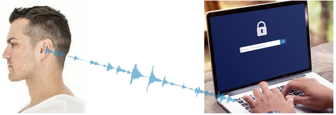
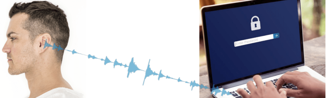
To be more specific (see Fig. 1), can we figure out what someone is typing, just by listening to the keystrokes? As one can imagine, it has some serious security implications, e.g., hacking passwords.

So I worked on a project called kido (= keystroke decode) to explore if this was possible (https://github.com/tikeswar/kido).

Outline

This can be treated as a supervised ML problem, and we will go over all the steps.

1. Data Gathering, and Preparation
2. Training and Evaluation
3. Testing and Error Analysis (improving model accuracy)
4. Conclusions; GitHub Link

Used Python, Keras, and TensorFlow for this project.

Data Gathering

The first step is, how do we collect the data to train a model?

There are many ways one can go about it, but just to prove if this idea works or not, I used my MacBook Pro keyboard to type, and QuickTime Player to record the audio of typing through the inbuilt mic (Fig. 2).

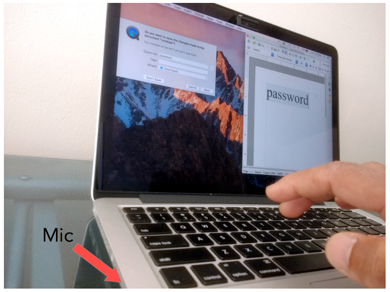
This approach has couple of advantages, 1. the data has less variability, and thus, 2. it helps us focus on proving (or disproving) the idea without much distraction.

Data Preparation

The next step is to prep the data so that we can feed it to a Neural Network (NN) for training.

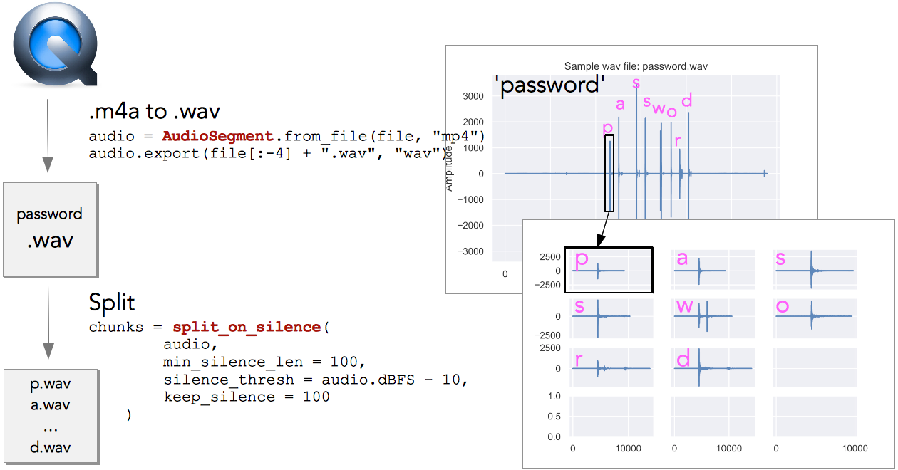
Quicktime saves the recorded audio as mp4. We first convert the mp4 to wav, as there are good Python libraries to work with the wav files. Each spike in the top-right subplot corresponds to a keystroke (see Fig. 3). Then we split the audio into individual chunks using silence detection, so that each chunk contains only one letter. Now we could feed these individual chunks to a NN, but there is a better approach.

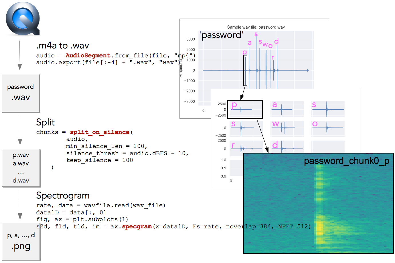
We convert the individual chunks into spectrograms (Fig. 4). And now we have images that are much more informative and easier to work with using a Convolutional Neural Network (CNN).

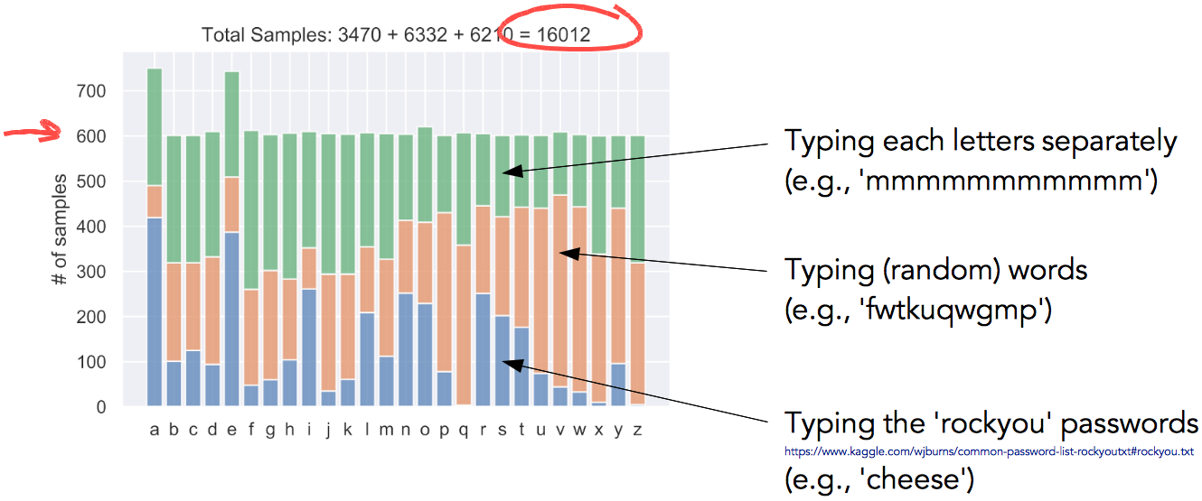
To train the network I collected about 16,000 samples as described above, making sure each letter had at least 600 samples (Fig. 5).

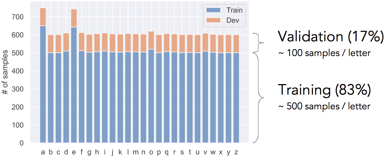
Then the data was shuffled and split into training and validation sets. Each letter had about 500 training samples + 100 validation samples (Fig. 6).

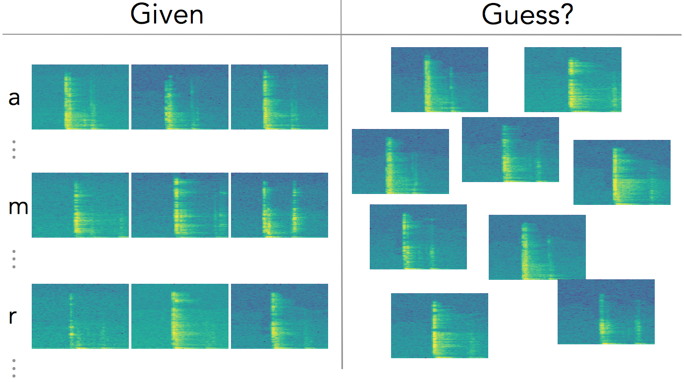
So, in a nutshell, this is the ML problem we have … see Fig. 7.

Training and Validation

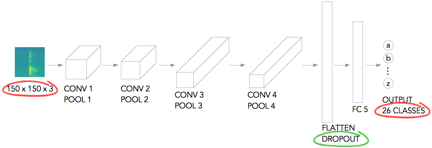
I used a fairly small and simple network architecture (based on Laurence Moroney’s rock-paper-scissor example). See Fig. 8 — the input image is scaled to 150 x 150 pixels, and it has 3 color channels. Then it goes through a series of convolution + pooling layers, gets flattened (used dropout to prevent over-fitting), gets fed to a fully-connected layer, and the output layer at the end. The output layer has 26 classes, corresponding to each letters.

In TensorFlow the model looks like:

model = tf.keras.models.Sequential([
    # 1st convolution
    tf.keras.layers.Conv2D(64, (3,3), activation='relu', input_shape=(150, 150, 3)),
    tf.keras.layers.MaxPooling2D(2, 2),    # 2nd convolution
    tf.keras.layers.Conv2D(64, (3,3), activation='relu'),
    tf.keras.layers.MaxPooling2D(2,2),    # 3rd convolution
    tf.keras.layers.Conv2D(128, (3,3), activation='relu'),
    tf.keras.layers.MaxPooling2D(2,2),    # 4th convolution
    tf.keras.layers.Conv2D(128, (3,3), activation='relu'),
    tf.keras.layers.MaxPooling2D(2,2),    # Flatten the results to feed into a DNN
    tf.keras.layers.Flatten(),
    tf.keras.layers.Dropout(0.5),    # FC layer
    tf.keras.layers.Dense(512, activation='relu'),    # Output layer
    tf.keras.layers.Dense(26, activation='softmax')
])

and the model summary:

_________________________________________________________________
Layer (type)                 Output Shape              Param #   
=================================================================
conv2d_4 (Conv2D)            (None, 148, 148, 64)      1792      
_________________________________________________________________
max_pooling2d_4 (MaxPooling2 (None, 74, 74, 64)        0         
_________________________________________________________________
conv2d_5 (Conv2D)            (None, 72, 72, 64)        36928     
_________________________________________________________________
max_pooling2d_5 (MaxPooling2 (None, 36, 36, 64)        0         
_________________________________________________________________
conv2d_6 (Conv2D)            (None, 34, 34, 128)       73856     
_________________________________________________________________
max_pooling2d_6 (MaxPooling2 (None, 17, 17, 128)       0         
_________________________________________________________________
conv2d_7 (Conv2D)            (None, 15, 15, 128)       147584    
_________________________________________________________________
max_pooling2d_7 (MaxPooling2 (None, 7, 7, 128)         0         
_________________________________________________________________
flatten_1 (Flatten)          (None, 6272)              0         
_________________________________________________________________
dropout_1 (Dropout)          (None, 6272)              0         
_________________________________________________________________
dense_2 (Dense)              (None, 512)               3211776   
_________________________________________________________________
dense_3 (Dense)              (None, 26)                13338     
=================================================================
Total params: 3,485,274
Trainable params: 3,485,274
Non-trainable params: 0

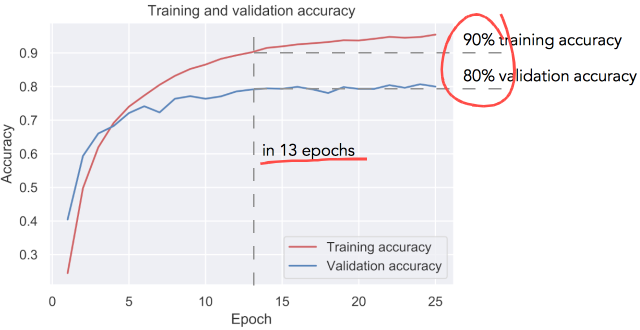
The training result is shown in Fig. 9. In about 13 epochs it converges to 80% validation accuracy with 90% training accuracy. I was pleasantly surprised to get this level of accuracy, given the complexity of the problem and simple network architecture used.

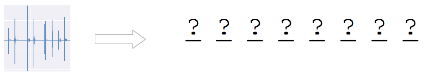
The result so far looks very promising … but, please note that this is character-level accuracy, not word-level accuracy.

What does that mean? In order to guess a password, we have to predict every single characters right, not just most of them right! See Fig. 10.

Testing

So, in order to test the model I digitized another 200 different passwords from the rockyou.txt list, and then tried to predict the words using the model we just trained (Fig. 11).

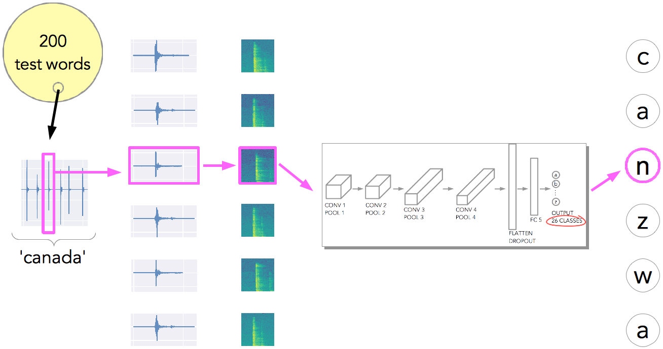
Fig. 12 shows the test accuracy. The bar charts show character-level accuracy (the left chart shows number of right and wrong, while the right chart shows the same in percentage). The test accuracy is about 49% for character-level and 1.5% for word level (the network got 3 out of the 200 test words completely right).

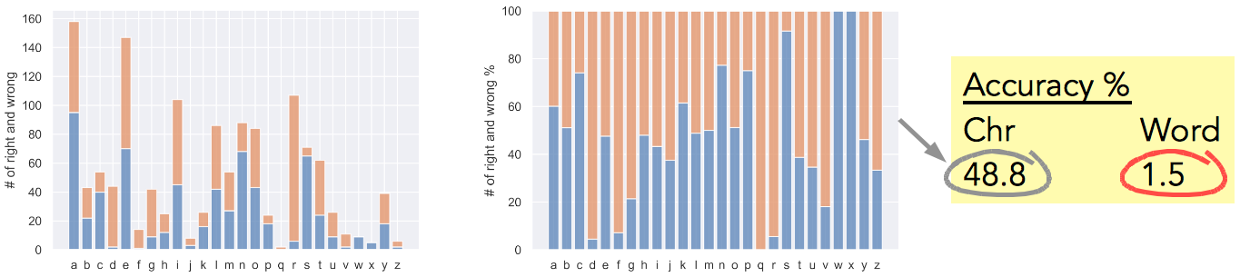
Given the complexity of the task, 1.5% word-level accuracy is not bad! But can we improve the accuracy?

Error Analysis

Let’s analyze the individual errors, and see if there are ways we can improve the prediction accuracy.

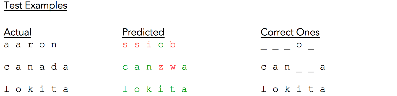
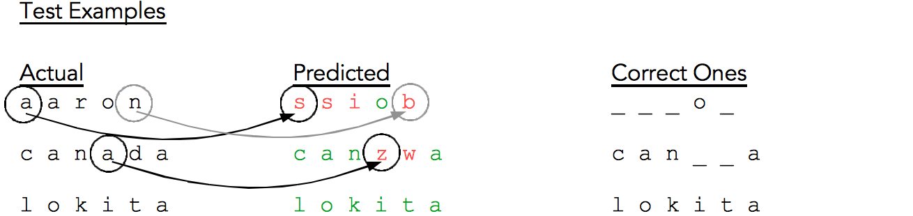
Fig. 13 shows some sample test results. The first column contains the actual test words, the middle column contains the respective predicted words where individual characters are color coded to show right (green) and wrong (red) predictions. The third column only shows the correctly predicted characters with the incorrectly predicted characters replaced by an underscore (for easier visualization).

For the word ‘aaron’ our model gets barely one character right, for ‘canada’ it gets most of the characters right, and for ‘lokita’ it gets all characters right. As mentioned in Fig. 12, word-level accuracy was only 1.5%.

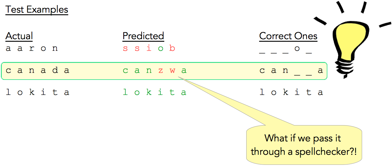
Squinting at the test examples (Fig. 14), especially ‘canada’, we realize it gets most of the characters right and is very close to the actual word. So, what if we pass the CNN result through a spellchecker?!

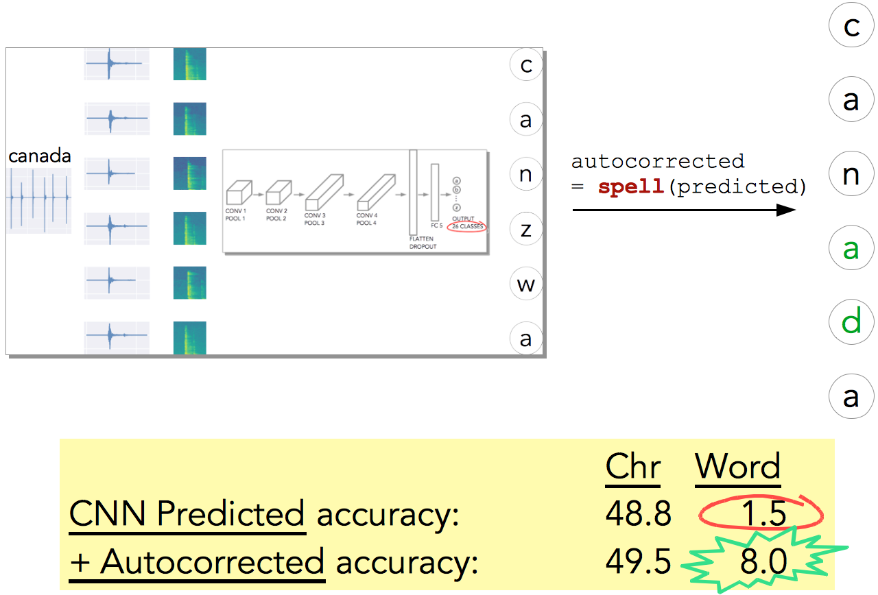
This is precisely what I did (Fig. 15), and sure enough it boosted the accuracy from 1.5% to 8%! So with a fairly simple model architecture + spellchecker we can predict 8 out of 100 passwords correctly … this is nontrivial!!

I think if we employed a sequence model (RNN?, Transformer?), instead of a simple spellchecker, we can get even higher word-level accuracy … and this can be a topic for further studies.

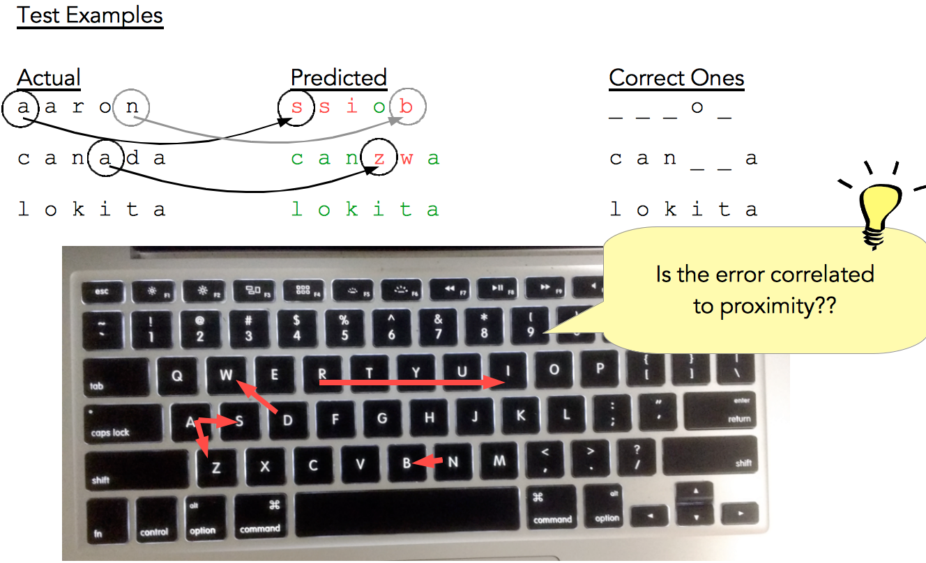
But let’s look even more closely at the test results (Fig. 16). We notice that ‘a’ gets predicted as ‘s’, ’n’ as ‘b’, etc.

So what if we map the errors on the keyboard? And once we have that mapped (see Fig. 17), is the error correlated to proximity? It seems like!

Next, can we quantify this error correlation with proximity?

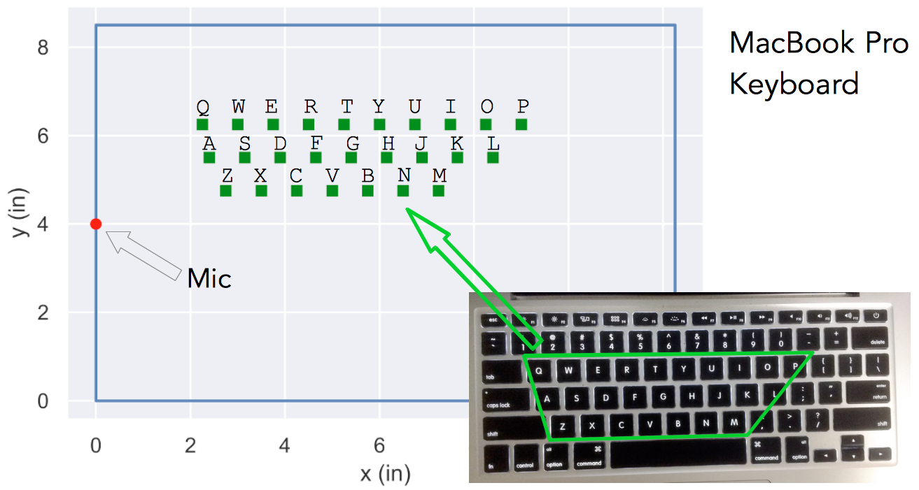
Fig. 18 shows the MacBook Pro keyboard with the mic and the key locations plotted to scale. Fig. 19 shows the error maps on the digitized keyboard for some sample letters.

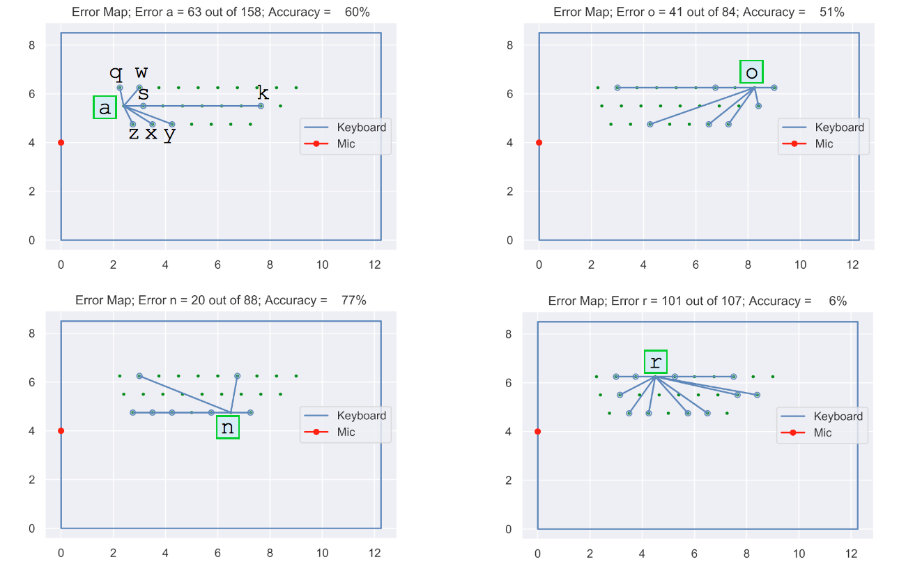
In Fig. 19, the top-left plot shows that ‘a’ gets wrongly predicted as ‘z’, ‘x’, ‘y’, ‘k’, ‘s’, ‘w’, or ‘q’. The other sub-plots are interpreted similarly.

Fig. 19 gives a more clear indication that the error may be correlated to proximity. However, can we get a even more quantitative measure?

Let d_ref be the distance of the reference letter from the mic, d_predicted be the distance of the predicted letter from the mic, and d be the absolute value of the difference between d_ref and d_predicted (see Fig. 20).

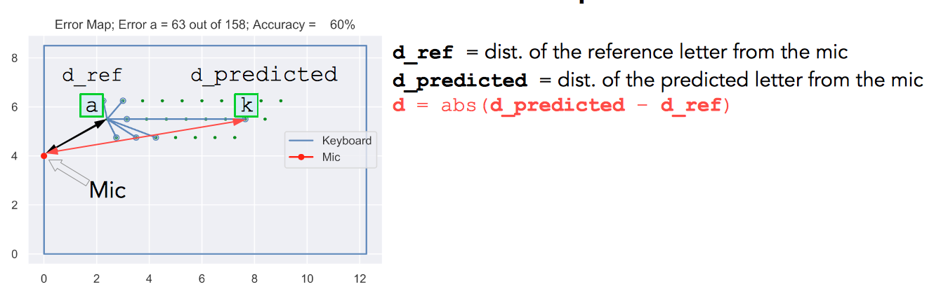
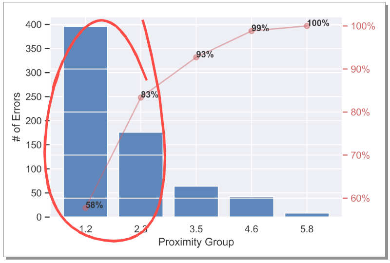
Fig. 21 shows histogram of the number of errors binned w.r.t. d. We see a very clear trend — most errors are from the close proximity! This also means we can probably improve the model accuracy with more data, bigger network, or a network architecture that can capture this better.

But what about the mic location — is the error correlated to how far a key is from the mic? To investigate this, the % error plot from Fig. 12 was rearranged such that the letters on the x-axis are in the increasing order of distance from the mic (see Fig. 22). No strong correlation is seen here w.r.t. d_ref, indicating the errors are independent of the mic location.

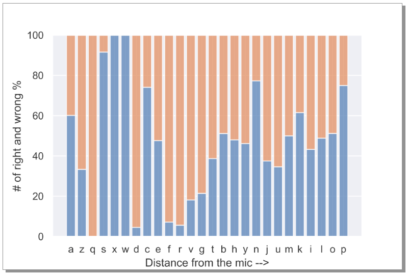
Fig. 22 highlights a very important point — one can place a mic anywhere to listen to the keystrokes and be able to hack! Creepy!

Model Enhancements

For this study I had made some simplifications just to see if the idea of hacking simply by listening to the keystrokes works. Following are some thoughts on improving the model to handle more complex and real-life scenarios.

• Normal typing speed → Challenging signal processing (to isolate individual keystrokes). — For this study I had typed slow one letter at a time.
• Any keystrokes → Challenging signal processing (Caps Lock on?, Shift?, …). — For this study I had used only lowercase letters (no uppercase letters, digits, special characters, special keystrokes, etc. were included).
• Background noise → Add noise. — For this study, during the data recording some simple and light background noise of cars passing by were present in some cases, but no complex background noise (cafeteria background noise for example).
• Different keyboards and microphone settings + different persons typing → More data + data augmentation + bigger network + different network architecture may help improve the model.
• → Can we use other vibration signatures instead of the audio signature?

Conclusions

Keeping in mind the simplifications made for this study,

• It seems possible to hack the keystroke sounds
• With a fairly small amount of data and a simple CNN architecture + spellcheck, we can get a non-trivial word-level accuracy (8% in this study)
• Error analysis
  * A simple spellcheck can boost word-level accuracy (from 1.5% to 8% in this case)
  * Errors correlate with proximity to the other keys
  * Errors seem independent of the mic location

All Rights Reserved for Tikeswar Naik